
Cryptocurrency Portfolio Management: The Deep Reinforcement Learning Approach
Alon Zabatani
Supervised by Tom Zahavy
Portfolio Management
Portfolio Management is the decision-making process of allocating wealth across a set of assets, it is a fundamental problem in computational finance, which has been extensively studied across several research communities, including
finance, statistics, machine learning, data mining, etc.
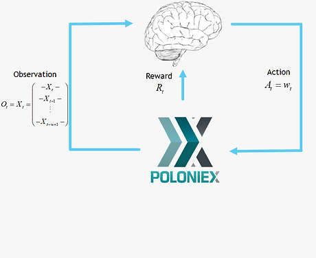
Reinforcement Learning
Deep Reinforcement Learning
Deep Reinforcement Learning has received considerable attention in recent years, it has shown remarkable achievements in playing video games [Mnih et al. (2013)] and board games [Silver et al. (2017)].
These are problems with discrete action spaces, and can not be directly applied to the portfolio management problem, where actions are continuous.
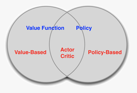
Policy-Based Methods
Direct parametrization of the policy (a DNN in our case).
Some of the advantages:
Effective in high-dimensional continuous action spaces
Better convergence properties
Data
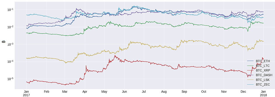
We collected historical data of 2017 from the Poloniex.com exchange.
The data consisted of the following coins: Ethereum (ETH), Litecoin (LTC), Ripple (XRP), Dash (DASH), Lisk (LSK) and Zcash (ZEC).
For each of the 6 coins, we collected opening prices in time intervals of 30 minutes. The prices are in Bitcoin, this implicitly makes Bitcoin our riskless asset and we thus end up with 7 coins in total.
We also assumed a transaction fee (both for selling and buying) of 0.25%, which is the maximal fee on Poloniex.com.
We divided our yearly data into quarterlies, we trained the agent on the first two months of each quarterly (2,880 samples), where 20% of it was used for validation, and then tested its performance on the following two weeks (672 samples).
For example, in the first quarterly we trained on 01/01/2017 - 01/03/2017 and then tested on 01/03/2017 - 14/03/2017.
We made two assumptions about our data:
1. Market Liquidity: we assume that one can buy and sell any quantity of any asset in its opening price
2. Zero Impact: we assume market behavior is not affected by our strategy
Method
Formalism
Problem setting

Network Architecture
Convolutional Neural Networks (CNNs) are known to be powerful tools for capturing spatially invariant patterns
[Krizhevsky, Sutskever, and Hinton (2012); Van Noord and Postma (2017)]. In sequential data for example, they can uncover recurring patterns like weekly cyclically or certain auto-correlation structures. CNNs are also usually easier to train than Recurrent Neural Networks (RNNs) and can outperform them in various tasks [Bai, Kolter, and Koltun (2018)].
Our CNN is used on the scaled asset price matrix (we separately scaled each column of the asset price matrix into the range [0,1]) as a "feature extractor". The extracted features are flattened and concatenated to the current portfolio vector, this makes the the agent "aware" of its current standings with hope that notions like transaction fees will be learned and accounted for. After a couple of fully-connected layers, a Softmax layer is used to output an action.

REINFORCE Algorithm
The Zero Impact assumption we introduced earlier dictates that the environment state is completely independent of the agent actions (quite uncommon in traditional RL problems), which is a reasonable assumption considering the relatively small sums we are moving. This allows us to split the environment into equally-long trajectories, each of length T.
The network is then trained in a fashion that resembles the well-known REINFORCE algorithm, in the sense that we play a trajectory and then take a gradient step in a direction that optimizes a certain objective. In our case each, the objective is the exponential growth rate and so we define the minus of it as our loss function:

Model Selection
Model selection is the task of selecting a statistical model from a set of candidate models, given data, and is usually done by dividing the data into two sets: training and validation. The validation set is the set of examples used for model selection. The validation set provides an unbiased evaluation of each model fit on the test set, used to compare performance of the different models and decide which one to use (e.g., choosing the number of hidden layers in a neural network).
In our online scenario, the best choice for validation set would be the most recent observations, as they are
usually more highly correlated with the test set (remember that we’re dealing with a time series). However, the most
recent observations are also our most valuable resource and ideally we would like our model to train on them. This poses a problem.
The most prevalent method to overcome this is to train on the whole dataset (train and validation) after a model has been selected. It has been demonstrated by Cawley and Talbot (2010), that such incorrect use of the validation set can lead to a misleading optimistic bias, resulting in an unreliable choice of model.
Tennenholtz, Zahavy, and Mannor (2018) recently showed that the requirement of a segregated validation set can be relaxed under stability assumptions of the learning algorithm (unfortunately, neural networks have not yet been shown stable).
In their work they introduced the batch-sample procedure, where at each training iteration, a batch is either taken from the train set or the validation set, independently of other batches. In our case, a batch is simply a set of trajectories.
An example of the procedure results when searching for the optimal Window Size are shown below:

Results
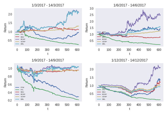
We tested our model against the following baselines:
Follow The Winner (FTW) - Invests all wealth in the recent best performing asset
Follow The Loser (FTL) - Invests all wealth in the recent worst performing asset
Buy And Hold (BAH) - Chooses an initial portfolio vector with no rebalancing in the future
Uniform Constant Rebalanced Portfolio (UCRP) - Rebalances the portfolio vector to a uniform vector
Best Constant Rebalanced Portfolio (BCRP) - Rebalances the portfolio vector to the optimal vector in hindsight
Results are shown below, each graph represents the test cumulative return as a function of t, in different quarterlies of 2017. Our algorithm is denoted as DRL and competes against the above baselines. As can be seen, our algorithm is always profitable. On the top left for example, the plot represents the first two weeks of March 2017 where DRL achieves a 2.076-fold return.
Conclusion
We developed a model-free, policy gradient algorithm based on a CNN and a full exploitation of the explicit reward function.
We used a novel method for model selection that allowed controlled sampling of validation data. Since we
were dealing with temporal data, where the most recent observations are crucial to both training and validation, this proved to be a very powerful tool (e.g., in 2017Q2, we more than doubled our final return, from 0.741 without validation sampling to 1.575 with it).
The final result is a robust, profitable algorithm, that never losses (even in scenarios where the entire market goes down, 2017Q3) and achieves up to a 2-fold return in a period of 14 days (2017Q1).